Classification model differentiation!!!……

Overview
Here I analyzed the return dispatches of field force and their leading cause of the returns for one of the telecom providers in US.
I got a proprietary service dispatch data from one of the telecom service provider which is used for academic purpose. I got total 12 months of 2019 service dispatch dataset as ‘.csv’ format.
FFE (Field Force Enablement) is a system that combines processes and services to support companies in locating field force, managing their activity, schedule and dispatch work and integrate with inventory, billing, accounting and other back office systems. This tool is most commonly used by the companies which need to manage installs, service or repairs of the systems or equipment.
FFE plays a pivotal role in making sure that telecom operations run smoothly 24 hours a day 365 days a year. A singular error can affect millions of people not to mentions thousands of business that are ever reliant on telecommunication to run their operations on a daily basis.
To begin exploring the problem first I checked the dataset as some features are not useful for predictions.I decided to drop those features as it will not impact to my dataset. Then I started to check null values or any missing values in the dataset. After checking the amount of null values (missing values) which are in the features ,I decided to drop these.
Then I started to do EDA(Exploratory data Analysis) on my dataset. There I noticed Job types , Location density and regions showing significant effect on the dataset. Considering all these features ,total 17 features I decided to take as my independent variable against my target variable. Then I split my dataset and fit my variables in a different classification models. As dataset now contained total 57 features I decided to Apply PCA(Principal Component Analysis) first to get the variance of the data and PCA also use for dimensional reduction.
Confusion matrix shows K Neighbor classification model shows 99% accuracy score on my datasets. After that I tried to find predictive classification model for the return statement code which signifies the major return caused. SVM(Support Vector machine) shows 96% accuracy score into my dataset.It is a very good score ,it means that the classifier has 96% chance of correctly classifying a new unseen example.
Goal
Developed a model for Field Technicians of largest US Telecom service provider to predict the probability of a job being returned at the time of assignment to ensure that the corrective actions are taken to avoid the return
Data Acquisition
Proprietary service dispatch data (Use for academic purposes)
Data Cleaning
Next I tried to clean all the data and labelling them, as most of the features are categorical. Data sets contain total 1658098 index with 244 features. Most of the features contain only one value. I dropped all those features value as this will not carry any information to my dataset. It becomes 74 features. Then I checked missing or null values and I decided to drop all the null values as my dataset will not lose any valuable information from this.
Exploratory data Analysis
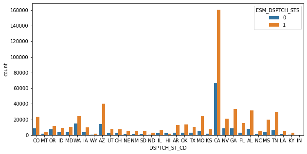
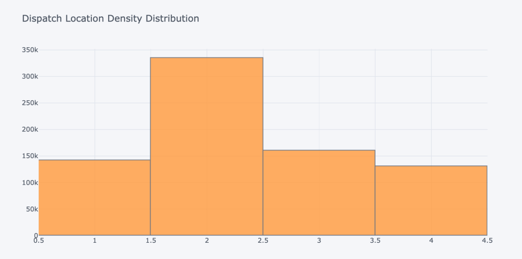
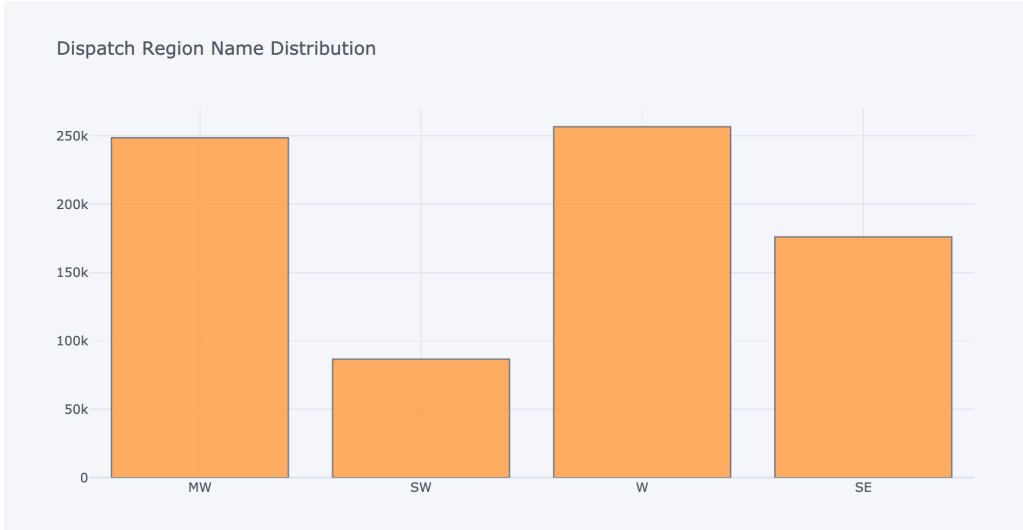
As all the data are categorical, try to find their distribution through interactive plot by ‘plotly.graph_objs’ library. Job type and location and location density and region name showing significant impact on the data.Below you can see their plots
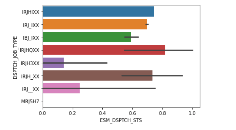
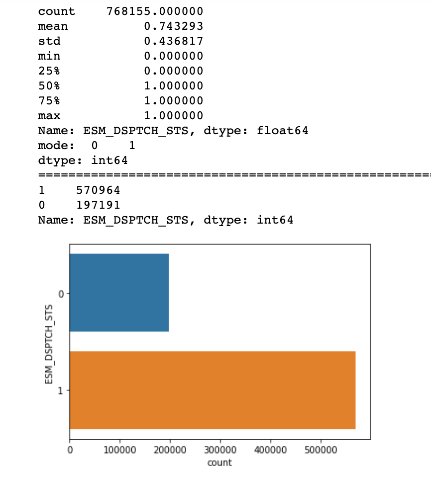
Mostly all the features are categorical, so I made dummies of each features,to get the numeric values.My dataframe becomes now 57 features (columns) and 1658098 (rows). Then I classified My target features which had a balanced of classes of 57% for class 1(Job Complete) and 20% for class 0(Job return)
Then I decided to split my data set into two splits training data sets and test data set. As my datasets contain large number of features, it may gives high variance to the model so I decided to apply PCA(Principal Component Analysis ) to get the variance of the data and PCA also use for dimensional reduction.
Model fitting and evaluate model
Before applying PCA I scaled my data set.
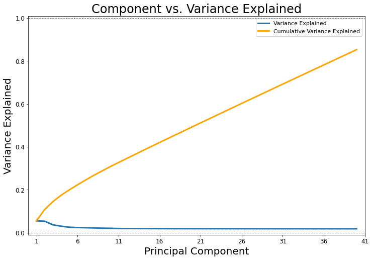
PCA plot: Percentage of variance of each feature.
It shows that the first component has the highest variance, something value around 10% while the 5th component is around of 0% of variance. So, it indicates that we should pick up the first five components. The second figure show another perspective of the variance, though the cumulative sum over all the variance, you can see that the first five eigenvalues correspond to approximately 85% of the all variance. Indeed, it is a pretty good number, it means that there is just 15% of information being lost. The biggest beneficial is that we are moving from a space with fifty-seven features to another one with only five features losing only 15% of information. That is the power of dimensionality reduction, definitively. Below you can see PCA plot of the dataset.
Confusion matrix classification shows first five principal components giving 85% accuracy score in logistic regression, Random Forest Classifier shows 88% accuracy and K Neighbor classifier gives 99% accuracy which is very much good prediction score. It means that the classifier has 99% chance of correctly classifying a new unseen example.
Second Model
Next I tried to predict model for the return statement code which signifies the major return caused.
Model fitting and evaluate model
From the datasets I extracted return dispatchment code and labelled them as numeric code. Python has a label encoder library, which can use for features labelling.
I made all features as dummies variable as, mostly are categorical. First, I applied PCA on independent features to get variance of the features. Considered first 3 components as my training data sets and predicted the value on the test data set.
My Logistic regression classification model gives accuracy rate 63 % where Support Vector Machine gives 96% accuracy. Support Vector machine gives good performance on predictions of multi classifications variable.It means that the classifier has 96% chance of correctly classifying a new unseen example.
Findings and Recommendations
As whole data set, we can say only some portion of company’s data information. There are many other factors depend on this. I try to predict which are the main features those can impact to analyze the data and to predict the return cause. From the data set we can say region and location state showing high impact on my model. Particular job types also showing difference to my model. Second model showing that mainly customer requested delay and customer not at home codes gives big impact on dataset.
And lastly, I would recommend following three things to the company
- I can say My model will predict future of any particular job, which will get returned or not.
- I will recommend to the company that customer presence at home should check before starting the dispatchment as most of the return code showing this reason
- And also equipment requirement means correct equipment should check before the dispatchment otherwise that job will get returned which is loss for the company.
